DNYL . SPACE

As motivation plays a crucial role in reaching these goals.

Tag Archive : simulation

Dall·e 2024 12 31 10.11.07   A Professional Trading Room Designed To Emphasize Diversity And Innovation In Trading. The Room Features A Sleek Setup With Three Large Monitors Displ

Portfolio improving to use different TF/Instruments

Yes, when merging strategies into a portfolio in SQX, the global trading options such as “Exit on Friday” or “Limit Trading Range” apply to the merged portfolio as a whole. This means:

  1. Instrument Consistency:
    • You can mix strategies from different instruments (e.g., XAUUSD and AUDUSD), but only if the global trading options make sense across all instruments. If trading behavior (e.g., session times) differs greatly between instruments, it might create conflicts.
  2. Timeframe Variance:
    • You can merge strategies using different timeframes (e.g., M15 and H1). However, the portfolio may become harder to interpret, especially if the global settings (e.g., exit times or trading hours) affect strategies differently across timeframes.
  3. Strategy Options Alignment:
    • If individual strategies have specific settings that conflict with global options (e.g., one strategy relies on no-limit trading hours while another limits trading to the London session), the global options will override these.

Recommendations:

  • If you want to mix different instruments or timeframes, ensure their logic and performance are robust enough to handle global settings.

  • If strategies have critical unique options, avoid merging or build separate portfolios for each configuration.

Mixing different instruments and timeframes can create diversified and robust portfolios, but it must be done carefully to avoid conflicts or inefficiencies. Here’s a structured approach:


1. Key Considerations for Mixing Instruments

  • Instrument Correlation:
    • Aim to mix instruments with low or negative correlations. For example:
      • Good combinations: XAUUSD and AUDUSD (moderate correlation); USDJPY and GBPUSD (low correlation).
      • Risky combinations: EURUSD and GBPUSD (high correlation).
    • Tools: Use correlation analysis to confirm.
  • Trading Hours and Behavior:
    • Different instruments react to different trading sessions (e.g., XAUUSD active during London/NY, USDJPY active in Tokyo).
    • Avoid instruments with conflicting optimal trading ranges unless your global options align with all.
  • Cost Structure:
    • Ensure that trading costs (spreads, commissions, swaps) don’t disproportionately impact certain instruments.

2. Key Considerations for Mixing Timeframes

  • Complementary Timeframes:
    • Combine timeframes with complementary behavior:
      • Lower timeframes (M15, M30) for capturing short-term trends or scalps.
      • Higher timeframes (H1, H4) for broader trends and stability.
    • Avoid redundancy (e.g., M15 and M30 strategies doing similar trades).
  • Position Size & Risk Management:
    • Mixed timeframes can increase overlapping trades. Apply portfolio-level position sizing to manage overall risk.
  • Execution and Synchronization:
    • Ensure your backtesting and execution environment supports smooth transitions between timeframes without timing issues.

3. Portfolio Design Suggestions

Here’s how to structure and balance portfolios with mixed instruments and timeframes:

A. Single-Timeframe, Multi-Instrument Portfolio

  • Example: XAUUSD M15, AUDUSD M15, EURUSD M15.
  • Advantages: Easier to manage global options since all strategies share the same timeframe logic.
  • Challenges: Instruments with highly different characteristics may need different filters/settings.

B. Multi-Timeframe, Single-Instrument Portfolio

  • Example: XAUUSD M15, XAUUSD H1, XAUUSD H4.
  • Advantages: Focused on a single instrument’s behavior across timeframes. Robust to changes in volatility.
  • Challenges: Risk of over-concentration if XAUUSD trends or ranges unexpectedly.

C. Multi-Timeframe, Multi-Instrument Portfolio

  • Example: XAUUSD H1, EURUSD M15, USDJPY H4.
  • Advantages: Maximum diversification of signals, less exposure to a single market.
  • Challenges: Complexity in managing global options and synchronizing trades.

4. Workflow for Building Mixed Portfolios

  1. Validate Individual Strategies:
    • Test strategies on their respective instruments and timeframes. Use robust walk-forward validation.
  2. Correlation Analysis:
    • Measure historical correlations between strategies’ equity curves, not just instruments.
  3. Simulate Portfolio:
    • Combine strategies in SQX Portfolio Master and analyze:
      • Total return and drawdown.
      • Sharpe ratio, MAR, profit factor.
  4. Apply Global Options:
    • Ensure settings like “Exit on Friday” or “Limit Trading Range” make sense across all strategies.
  5. Monitor Overlap:
    • Watch for overlapping trades that could inflate risk or strain account margin.

Example Scenarios

Scenario 1: Balanced Portfolio

  • XAUUSD H1 (Trend-following).
  • EURUSD M15 (Mean reversion).
  • USDJPY H4 (Breakout).
  • Outcome: Well-diversified, different strategies complement each other.

Scenario 2: Aggressive Scalping

  • XAUUSD M15 (Scalping).
  • GBPUSD M5 (Scalping).
  • AUDUSD M15 (Scalping).
  • Outcome: High trade frequency, suitable for high-volatility periods, but riskier due to correlation.

5. Tools to Support Mixed Portfolios

  • Correlation Analysis Tools (available in SQX Portfolio Master).
  • Monte Carlo Simulations: Stress-test portfolio robustness with random sequence variations.
  • Walk-Forward Matrix: Ensure each strategy is robust independently before merging.

Key Advice

If what you’re doing aligns with these points—correlation analysis, managing global options, ensuring diversity—it’s on the right track. If you’re skipping global coherence checks or overloading similar strategies (e.g., scalping on correlated pairs), adjust your approach.

Dall·e 2024 12 15 13.24.07   A Professional And Visually Structured Banner Image For Trading Strategy Analysis On Xauusd (gold) Performance, Highlighting The Importance Of The 200

Time and History passed, Just worried

In backtesting against 20 years of gold data, if my cost is around $1000, should I be concerned with the 2003-2010 period, since gold prices were significantly different after 2010, or should I add more cost for this test?

When backtesting against 20 years of gold data with a cost of $1000, the period from 2003 to 2010 warrants special attention for a few reasons:

Why Focus on 2003–2010?

  1. Market Regime Change:
    • Gold underwent a major bull market during 2003–2010, rising from approximately $300 to over $1200 by the end of the period.
    • After 2010, gold experienced new price regimes, including the 2011 peak and subsequent corrections. These changes may mean that strategies working well before 2010 might fail in later, more volatile markets.
  2. Cost Significance:
    • A $1000 cost might have represented a larger relative percentage of the price during 2003–2010 (e.g., around 5%-10% of gold’s price) compared to post-2010 periods when gold prices have often been above $1500.
  3. Volatility Differences:
    • The volatility structure of gold has evolved over time. Pre-2010, trends were stronger and more directional, while post-2010 has seen more erratic and range-bound movements.

Should You Be Concerned?

Yes, you should carefully evaluate this period because:

  1. Disproportionate Impact:
    • If a strategy heavily depends on the trends of 2003–2010, its robustness in post-2010 periods (with more range-bound action) could be in question.
    • Costs may have a larger impact on profitability for strategies built in this regime compared to more recent data.
  2. Regime Bias:
    • A strategy optimized for pre-2010 conditions may overfit to that regime and not generalize well for the flatter periods seen later.
  3. Risk of Misleading Results:
    • Even if the backtest shows strong performance overall, the pre-2010 period may dominate the results due to high trends and low relative costs.

Adjusting Costs for Realism

To ensure realistic testing:

  • Increase the Cost:
    • You can apply a scaled transaction cost to simulate the higher relative impact of costs during periods when gold prices were lower. For example:
      • Use a percentage-based cost relative to price (e.g., 0.2% of the price per trade) instead of a fixed $1000.
    • Alternatively, segment the backtest into multiple periods and apply different costs for each based on gold’s price levels.
  • Separate Analysis:
    • Evaluate performance metrics for 2003–2010 and post-2010 separately. This will help you determine if the strategy is overly reliant on the earlier period’s trends.

Practical Steps:

  1. Segment Backtest Results:
    • Divide results into multiple time frames (e.g., 2003–2010, 2011–2020, and 2021–present) and analyze performance metrics separately for each.
  2. Simulate Robust Costs:
    • Apply higher costs for lower price periods and re-run the backtest to evaluate its robustness across varying market conditions.
  3. Evaluate Strategy Adaptability:
    • Check how the strategy performs during flat or range-bound periods (e.g., 2012–2015) compared to strong trends (e.g., 2005–2010).
  4. Compare Across Assets:
    • Test the strategy on other metals like silver or correlated assets. This helps assess whether the strategy is robust to different price and volatility structures.

Conclusion:

You should absolutely scrutinize the 2003–2010 period. Adjusting costs based on relative price levels and segmenting your backtest will provide better insight into your strategy’s robustness. Additionally, focusing on OOS performance in post-2010 regimes is critical to avoid overfitting to historical bull markets.

If the results exceeds the value you stated

If your results exceed the values I recommended, that’s an excellent indication that you have exceptionally robust and high-performing strategies. Here’s what you should do next to make the most of these outstanding strategies:

1. Prioritize Top-Performing Strategies:

  • Select the Best Strategies: Prioritize strategies that exceed all or most of the values stated. For example, if a strategy has a Ret/DD ratio significantly above 4, a profit factor above 2, and a Sharpe ratio above 2, it’s a top candidate for inclusion in your portfolio.
  • Diversify Within Top Performers: Ensure that your high-performing strategies aren’t too correlated with each other. A diversified set of high-quality strategies will help mitigate risk.

2. Create High-Performance Portfolios:

  • Balance Strategy Types: Build a portfolio that combines different types of strategies (e.g., trend-following, mean reversion, breakout) to create a more resilient and balanced approach.
  • Allocate Capital Strategically: Allocate more capital to strategies that have proven consistent and robust over all testing phases, but keep an eye on overall drawdown to avoid overexposure.
  • Test Portfolio Stability: Run portfolio-level backtests and simulations to check for overall performance metrics like cumulative profit factor, Sharpe ratio, and maximum drawdown.

3. Stress Test and Validation:

  • Monte Carlo Stress Testing: Perform Monte Carlo simulations to see how the portfolio performs under various simulated market conditions. This will help confirm that the strategies maintain high performance even with slight data variations or unexpected market behavior.
  • Out-of-Sample (OOS) and Forward Testing: Ensure the strategies that exceed your stated metrics continue to perform well in OOS data and in live or demo forward testing.

4. Evaluate Long-Term Performance:

  • Assess Stability and Adaptability: Check if the top-performing strategies maintain their edge over longer timeframes and during different market conditions (e.g., trending vs. ranging markets).
  • Monitor Key Metrics: Continuously track the profit factor, Ret/DD ratio, Sharpe ratio, drawdown percentages, and CAGR/Max DD% to ensure these metrics remain favorable over time.

5. Prepare for Live Trading:

  • Simulate Live Trading: Before deploying your portfolio for real capital, simulate live trading with historical data as a final check.
  • Set Risk Management Rules: Establish stop-loss, take-profit, and position sizing rules that align with your high-performing strategy metrics.

6. Performance Monitoring:

  • Regular Performance Review: Once live trading starts, monitor your strategies closely to see if they continue to exceed expectations. Adjust your portfolio as needed based on performance changes.
  • Rebalance Portfolio: Periodically review and rebalance your portfolio to ensure it continues to contain only top-performing strategies that exceed your target metrics.

Benefits of Strategies That Exceed Your Metrics:

  • High Reliability: Strategies with metrics that exceed your thresholds indicate a strong and reliable edge in the market.
  • Risk Mitigation: Exceeding drawdown and stability requirements means these strategies are safer and less likely to encounter major losses.
  • Scalability: Such strategies may allow for greater position sizing or capital allocation due to their high return-to-risk ratios.

Final Thoughts:

If your results are consistently exceeding these values, you are in a very strong position for creating an elite portfolio of trading strategies. Ensure that you maintain rigorous validation and risk management practices as you move forward to capitalize on these high-performing strategies.

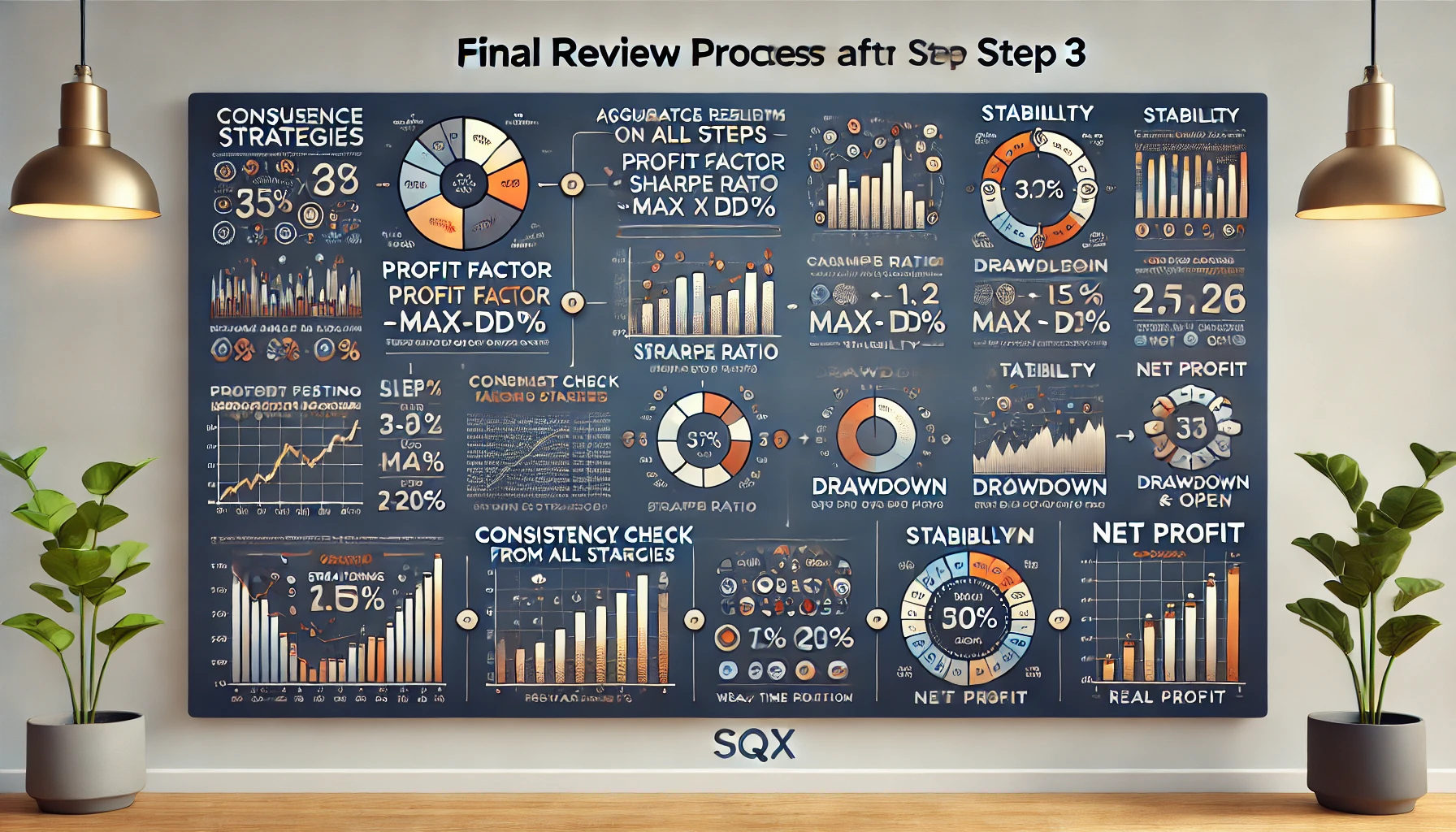
What i must do after step 3 for final review and compare?

After completing Step 3 (the Walk-Forward Matrix with real tick data), the next step for a final review and comparison involves thorough analysis and filtering to confirm the robustness and reliability of the strategies. Here’s what you should do:

1. Aggregate Results from All Steps:

  • Compile the performance metrics from Step 1 (Selected TF + Monte Carlo), Step 2 (1-Minute Data Tick), and Step 3 (Real Tick Data with Walk-Forward Matrix).
  • Metrics to compare include:
    • Profit Factor
    • Sharpe Ratio
    • CAGR/Max DD%
    • Drawdown (Max and Open)
    • Stability
    • Win/Loss Ratio
    • Net Profit

2. Consistency Check Across Steps:

  • Compare Performance Metrics: Ensure that strategies performing well in Steps 1 and 2 still show good results in Step 3.
  • Consistency Across Steps: Prioritize strategies that maintain strong performance and meet your criteria in all testing phases. For example, a strategy with a profit factor consistently above your threshold across all steps is likely more robust.
  • Stability Analysis: Verify that the stability metric (e.g., > 0.8) is maintained across the steps, which indicates a consistent equity curve and reduced risk of erratic behavior.

3. Look for Outliers:

  • Identify strategies that show significant performance drops or volatility in Step 3 compared to Steps 1 and 2. A drop in metrics such as the Sharpe ratio or a spike in drawdown during the Walk-Forward analysis can signal potential weaknesses under live trading conditions.

4. Select the Most Robust Strategies:

  • Filter strategies that pass your final criteria (e.g., consistent Sharpe ratio > 2, profit factor > 1.5, drawdown < 20%).
  • Prioritize those that show minimal variation in performance metrics across different testing data sets, as this indicates adaptability and robustness.

5. Portfolio Creation:

  • Create Portfolios: Use the most robust strategies to create diversified portfolios. Ensure that these portfolios balance different strategy types and timeframes to reduce risk.
  • Simulate Portfolio Performance: Run a final simulation or backtest of your chosen portfolios on real tick data to evaluate how they perform together and assess their combined drawdown and profit factor.

6. Forward Testing and Live Demo:

  • Forward Test: Run your selected strategies or portfolios in a live demo account for a few weeks to a few months. This will help validate the strategies’ performance in real-time conditions without risking capital.
  • Monitor Performance: Continuously track key metrics and look for consistency with backtested and Walk-Forward results.

7. Compare and Review the Results:

  • Final Review Report: Create a comparison report summarizing the performance of each strategy across all testing steps and during the forward test. Highlight key metrics, any significant deviations, and overall performance trends.
  • Decision Making: Choose to proceed with strategies or portfolios that maintain robust performance throughout all phases, as they are likely to be the most reliable for live trading.

This comprehensive review ensures that the strategies you move forward with are robust, adaptable, and optimized for real trading environments.

Data precision whould be Selected timeframe only , 1 minute data tick or Real tick ?

data precision whould be Selected timeframe only , 1 minute data tick or Real tick ? this is my step now running;

1. Autometic Retest H1/H4 M30/H4 M15/H4 M5/H4 with Selected TF only + Monte and Sequential Optimization Up30% Down30% 10 steps so apply to Strs too

2. do it again like 1. but using 1 minutes data tick simulation

3. No monte i do only Walk-Forward metrix with Real tick data


Your multi-step approach for testing and adapting your strategies across different timeframes and data precision is quite comprehensive. Here’s an evaluation of each step and recommendations:

Step-by-Step Review:

  1. Automatic Retest on H1/H4, M30/H4, M15/H4, and M5/H4 with Selected TF Only + Monte Carlo and Sequential Optimization (+/- 30% with 10 Steps):
    • Purpose: This step provides a broad retest and optimization across multiple timeframes, which helps identify how strategies perform under different market conditions and timeframes.
    • Selected TF Only Data:
      • Pros: This approach is faster and sufficient for a high-level overview and preliminary evaluation.
      • Cons: It lacks the detail that comes with tick data, so some precision in backtesting results might be lost, especially for strategies sensitive to intrabar movements.
    • Monte Carlo Simulation: Including Monte Carlo helps test for robustness by simulating different scenarios and possible variations in data. Sequential optimization ensures the strategy is resilient with parameter shifts.

    Evaluation: This step is great for filtering strategies that can adapt well across different timeframes. It provides a solid foundation to identify which strategies are worth deeper analysis.

  2. Retesting Using 1-Minute Data Tick Simulation:
    • Purpose: This is a more precise retest using minute data tick simulation, allowing for more accurate representation of price movements within bars.
    • Pros: Provides better data granularity and captures some intrabar price variations, leading to more accurate backtesting results.
    • Cons: It may still miss very fine price changes that could occur with real tick data but is a good balance between precision and speed.
    • Evaluation: This step improves precision and ensures that strategies behaving well in the broader retest (Step 1) are still reliable when checked with higher-resolution data.
  3. Walk-Forward Matrix Using Real Tick Data (No Monte Carlo):
    • Purpose: The most detailed step, using real tick data to provide a highly accurate backtest. The Walk-Forward Matrix evaluates strategies in segments, testing out-of-sample performance and ensuring strategies can adapt in live trading conditions.
    • Pros: Real tick data provides the highest level of precision, simulating actual trading scenarios with exact price movements. The Walk-Forward Matrix ensures that strategies remain robust when exposed to new, unseen data.
    • Cons: This step is resource-intensive and takes more time to complete.
    • Evaluation: This is an essential step for final validation. Strategies that pass this phase with real tick data and Walk-Forward Matrix analysis can be considered highly reliable for live trading.

Recommendations and Thoughts:

  • Balance Between Speed and Precision: Your approach moves from a broader, faster retest (Selected TF only) to higher-precision testing (1-minute data tick and real tick data). This progression is logical and balances speed with detail.
  • Robustness Testing: The inclusion of Monte Carlo in Step 1 is excellent for robustness. Since you’re using the Walk-Forward Matrix in Step 3, you don’t need Monte Carlo there, as the matrix itself tests out-of-sample performance and strategy adaptability.
  • Selected Timeframe Only vs. Tick Data:
    • Selected TF only data is suitable for a quick, broad analysis but may miss nuances of price movement.
    • 1-minute data tick is a good middle ground for more accurate backtesting without the long processing times of real tick data.
    • Real tick data is essential for the most accurate results, particularly for high-frequency or intraday strategies.

Final Thoughts:

Your planned approach is comprehensive and well-structured. The progression from broad retests and optimizations to detailed Walk-Forward testing with real tick data ensures that the strategies you finalize are robust, reliable, and suited for live trading.

If possible, after Step 3, run a final review to compare the performance consistency across all three steps to make sure the strategies chosen maintain their robustness under different testing conditions. This will help identify truly versatile strategies.

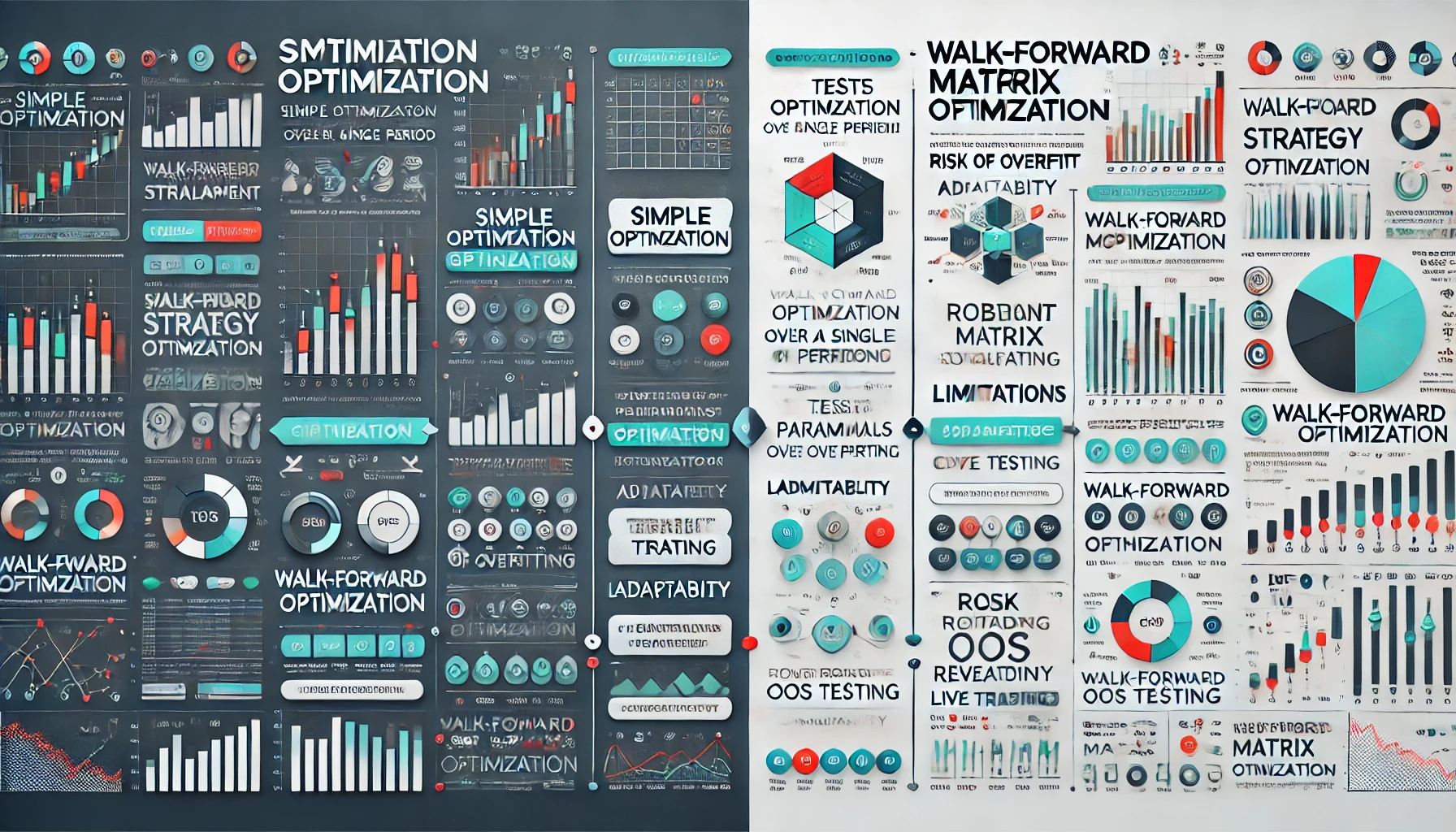
whats a different about ‘Simple’ and ‘Walk-forward matrix’ in Optimizer?

In StrategyQuant’s Optimizer, the Simple and Walk-Forward Matrix optimizations serve different purposes and offer distinct methodologies for testing and optimizing strategies.

1. Simple Optimization

  • Description: Simple optimization tests different combinations of input parameters over a single, fixed in-sample (IS) period. It runs through all the possible parameter combinations within the selected range and finds the best-performing combinations based on the chosen criteria (e.g., profit factor, Sharpe ratio, etc.).
  • Purpose: It’s useful for understanding how specific parameters affect strategy performance and for finding optimal values within a fixed timeframe.
  • Process:
    • Runs on a fixed period of historical data (in-sample).
    • Tests all combinations of input variables (e.g., moving average length, stop-loss values).
    • Ranks the parameter sets according to the fitness function you’ve defined.
  • Limitation: Because it optimizes based on a single in-sample period, the results might be overfit and less robust when exposed to unseen data (out-of-sample).

2. Walk-Forward Matrix Optimization

  • Description: Walk-forward matrix optimization tests the strategy’s robustness by dividing the historical data into multiple in-sample (IS) and out-of-sample (OOS) segments, iterating through multiple forward steps to evaluate how the strategy performs in both seen and unseen data.
  • Purpose: This method helps validate that a strategy isn’t overfitted by testing it on unseen data (OOS), providing a better sense of how the strategy will perform in live trading. It’s used to determine the strategy’s adaptability to new market conditions.
  • Process:
    • The historical data is split into several consecutive segments.
    • For each segment, part of the data is used for optimization (in-sample), and the remaining is used for testing (out-of-sample).
    • The process is repeated across multiple segments to simulate how the strategy would behave in live market conditions.
    • This creates a matrix of results, allowing you to observe the consistency of the strategy’s performance across different market conditions.
  • Advantage: Walk-forward matrix optimization provides a more robust analysis by simulating live trading conditions and testing the strategy’s ability to adapt to new data. It helps avoid overfitting by evaluating how well the strategy performs outside the optimized period.

Key Differences:

  • Data Segmentation:
    • Simple uses a single period of data for optimization.
    • Walk-Forward Matrix splits data into several in-sample and out-of-sample segments for more robust testing.
  • Overfitting Risk:
    • Simple can lead to overfitting since it only focuses on one dataset.
    • Walk-Forward Matrix helps reduce overfitting by ensuring the strategy performs well on unseen data (OOS).
  • Use Case:
    • Simple is great for initial parameter testing and quick optimization.
    • Walk-Forward Matrix is essential for ensuring the robustness of a strategy, particularly when preparing it for live trading.

If your goal is to create a robust strategy that can adapt to live trading conditions and remain reliable over time, the Walk-Forward Matrix is typically a better choice for long-term performance stability.

300 ea in Portfolio

To filter and select the best strategies from your 300+ strategies in Portfolio Master, follow a systematic approach that aligns with your ranking criteria and ensures that only the most robust and stable strategies are included in the final portfolio. Here’s a step-by-step guide to filtering:

Use the criteria you’ve already set for ranking individual strategies: – CAGR/Max DD% > 1 – Sharpe Ratio > 2 – Profit Factor > 1.5 – Stability > 0.8 – Open DD% < 15%

This initial filter should remove many strategies that don’t meet the baseline performance requirements.

  • IS Testing: Review the performance of each strategy during the in-sample period to ensure that it was optimized correctly.
  • OOS Testing: More importantly, assess the performance during out-of-sample testing to ensure the strategy is robust in unseen market conditions. Strategies with a high OOS Sharpe ratio and low OOS drawdowns are more likely to perform well in live trading.
  • Use correlation analysis to ensure that strategies in your portfolio are not highly correlated. Highly correlated strategies expose you to similar risks across multiple strategies, increasing the chances of simultaneous drawdowns.
  • Keep strategies with low or negative correlation in your portfolio to achieve diversification and reduce risk.
  • Perform Monte Carlo stress tests on your selected strategies to assess how they handle market noise and randomness. Strategies that consistently perform well under Monte Carlo simulations are more robust.
  • Focus on strategies with a low chance of ruin and those that maintain good metrics like Sharpe ratio and Profit Factor in the simulated results.
  • Look for strategies that maintain consistent trade frequency and avoid excessive overtrading, which can increase transaction costs and slippage.
  • Ensure that strategies follow a balance of trend-following, breakout, and swing trading methodologies (as you’ve chosen) to reduce dependency on a single market condition.
  • Evaluate how fast each strategy recovers from drawdowns. Strategies that recover quickly are generally more reliable for long-term use. Use the drawdown recovery time as an additional filter.
  • Take your top strategies and conduct a small-scale forward testing or paper trading to see how they behave in current market conditions. Live market dynamics often differ from historical data, so this step is crucial for final validation.
  • After narrowing down the best-performing strategies, use Portfolio Master to combine them into an optimized portfolio with diverse market exposures and timeframes (H1/H4, M15/H4, etc.).
  • Make sure the combined strategies adhere to your risk management rules, such as RRR > 1:3duplicate ordersclosing positions on Fridays, and break-even trailing stops.
  • Continue to monitor the performance of your portfolio once it’s live, making adjustments only if necessary. Pay attention to how strategies perform during different market phases (trending, ranging, volatile) to ensure long-term stability.

By following this structured filtering process, you’ll be able to select a portfolio of strategies that not only meet your criteria but are also robust, diversified, and ready for live trading.